Problem:
Suddenly, when turning your Dell laptop on you get the error message “Hard drive Not installed” and cannot boot into Windows.
Solution:
- Power your laptop and quickly press F2 key to enter BIOS.
- Expand System Configuration node.
- Click SATA Operation.
- If RAID option is being selected, select AHCI option.
- If AHCI option is being selected, select RAID option.
- Click Apply button.
- Click Exit button.
- If the problem still persists then restore BIOS settings to Default BIOS settings, then try the procedure again.
More information:
- PCI Express (Peripheral Component Interconnect Express), officially abbreviated as PCIe or PCI-e, is a high-speed serial computer expansion bus standard. It is the common motherboard interface for personal computers’ graphics cards, hard drives, SSDs, Wi-Fi and Ethernet hardware connections.
- NVM Express (NVMe) or Non-Volatile Memory Host Controller Interface Specification (NVMHCIS) is an open logical-device interface specification for accessing non-volatile storage media attached via PCI Express (PCIe) bus. By its design, NVM Express allows host hardware and software to fully exploit the levels of parallelism possible in modern SSDs. As a result, NVM Express reduces I/O overhead and brings various performance improvements relative to previous logical-device interfaces, including multiple long command queues, and reduced latency.
- Serial ATA (SATA, abbreviated from Serial AT Attachment) is a computer bus interface that connects host bus adapters to mass storage devices such as hard disk drives, optical drives, and solid-state drives.
- The Advanced Host Controller Interface (AHCI) is a technical standard defined by Intel that specifies the operation of Serial ATA (SATA) host controllers in a non-implementation-specific manner in its motherboard chipsets. AHCI is mainly recommended for SSDs that have better NVMe drivers from their factories.
- RAID (“Redundant Array of Inexpensive Disks” or “Redundant Array of Independent Disks“) is a data storage virtualization technology that combines multiple physical disk drive components into one or more logical units for the purposes of data redundancy, performance improvement, or both.
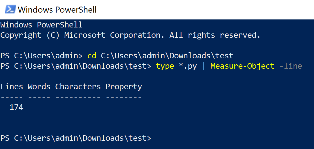
- AHCI mode uses Microsoft generic AHCI for standard SATA access. It is recommended for single-drive configurations and when using non-Intel NVMe or SATA SSDs. Use the PowerShell command below to get your SSD manufacture:
Get-PhysicalDisk | Select-Object FriendlyName, Manufacturer, Model, MediaType
- RAID mode uses Intel RST driver to leverage Intel firmware RAID and caching. It is recommended for multiple drives in a RAID array.
- If you switch from RAID to AHCI (or vice versa) after the OS is installed, Windows may fail to boot. That is because the required storage driver (AHCI or RST) was not active when Windows was installed.
- For a single SSD (especially NVMe), AHCI mode is slightly faster, but only by a few percent.