Context:
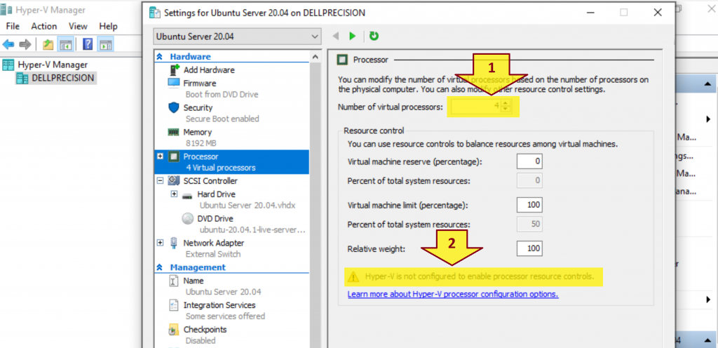
You got a warning message below when configuring Number of virtual processors in Hyper-V.
Hyper-V is not configured to enable processor resource controls.
Problem:
How do you enable processor resource controls in Hyper-V?
Solution:
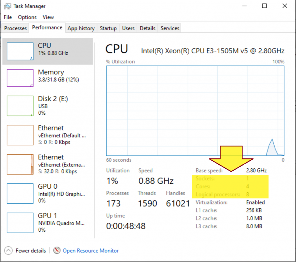
1. What is the difference between core and logical processor?
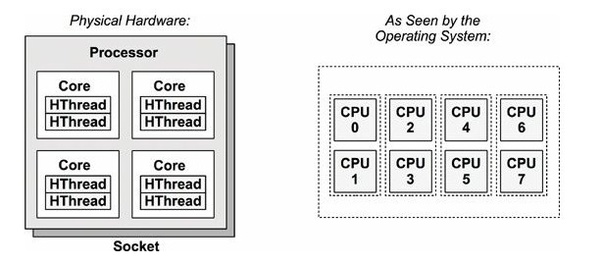
- A socket is a slot contains one or more mechanical components providing mechanical and electrical connections between a microprocessor and a printed circuit board (PCB). This allows for placing and replacing the central processing unit (CPU) without soldering.
- A core is a physical processor unit (hardware component) inside your processor.
- Logical processor or logical core is the processor as seen by the operating system. Logical processor does not exist physically.
Logical Processor = (# of Core) * (# of Thread in each Core) = 4 * 2 = 8
Example:
2. What is SMT?
Simultaneous multithreading, or SMT, is a technique utilized in modern processor designs that allows the processor’s resources to be shared by separate, independent execution threads.
Processors supporting SMT are available from both Intel and AMD. Intel refers to their SMT offerings as Intel Hyper Threading Technology, or Intel HT.
3. How does Hyper-V virtualize processors?
- Hyper-V creates and manages virtual machine partitions, across which compute resources are allocated and shared, under control of the hypervisor. Partitions provide strong isolation boundaries between all guest virtual machines, and between guest VMs and the root partition.
- The root partition is itself a virtual machine partition, although it has unique properties and much greater privileges than guest virtual machines. The root partition provides the management services that control all guest virtual machines, provides virtual device support for guests, and manages all device I/O for guest virtual machines. Microsoft strongly recommends not running any application workloads in the root partition.
- Each virtual processor (VP) of the root partition is mapped 1:1 to an underlying logical processor (LP). A host VP always runs on the same underlying LP – there is no migration of the root partition’s VPs.
- By default, the LPs on which host VPs run can also run guest VPs.
- A guest VP may be scheduled by the hypervisor to run on any available logical processor. While the hypervisor scheduler takes care to consider temporal cache locality, NUMA topology, and many other factors when scheduling a guest VP, ultimately the VP could be scheduled on any host LP.
4. What are Hyper-V hypervisor scheduler types?
Starting with Windows Server 2016, the Hyper-V hypervisor supports several modes of scheduler logic, which determine how the hypervisor schedules virtual processors on the underlying logical processors. These scheduler types are:
- The classic scheduler provides a fair share, preemptive round- robin scheduling model for guest virtual processors.
- The core scheduler offers a strong security boundary for guest workload isolation, and reduced performance variability for workloads inside of VMs that are running on an SMT-enabled virtualization host.
- The root scheduler cedes control of work scheduling to the root partition. The NT scheduler in the root partition’s OS instance manages all aspects of scheduling work to system LPs.
5. Determine your current Hyper-V Hypervisor Scheduler Type
Execute the command below.
Get-WinEvent -FilterHashTable @{ProviderName="Microsoft-Windows-Hyper-V-Hypervisor"; ID=2} -MaxEvents 1
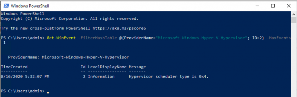
- 1 = Classic scheduler, SMT disabled
- 2 = Classic scheduler
- 3 = Core scheduler
- 4 = Root scheduler
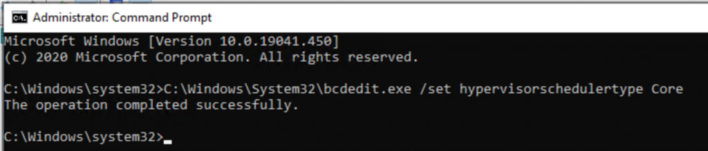
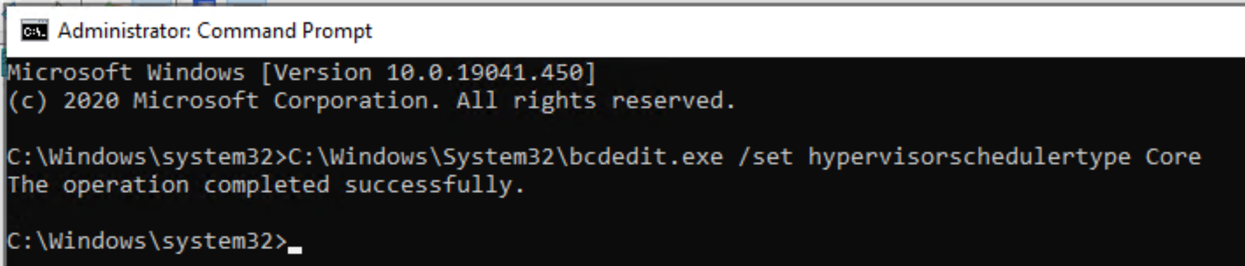
6. Enable processor resource controls in Hyper-V by setting Scheduler Type to Core or Classic.
- Open a Command Prompt as Administrator.
- Execute the command below.
C:\Windows\System32\bcdedit.exe /set hypervisorschedulertype Core